Introduction to R
Aiden Loe
07 January, 2021
How to start using R?
You got here because you are keen on learning R, so luckily, I don’t have to give you reasons to do so.
Here is the first question. How do you start using R? (Given that you have R and R studio in your computer)
Think of R as the engine of a car and R studio as the structure of the car.
In order for your car to work, you first need the engine. So, in order for R studio to work, you need R. Manipulation is done via R studio, and not R itself. Just like how you would want to accelerate faster or slower, listen to music or turn on/off the air-condition in the car, the functions are found in the interior of the car which is then connected to the engine. So the basic idea is, your working environment will be R studio.
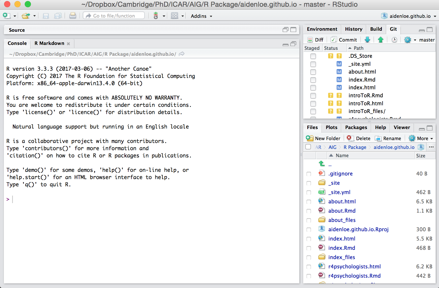
R studio
This is how it looks like the first time you open Rstudio.
Script and Console
The best way to work in R studio is to use a script. Click the ‘+’ sign on the top left of R studio and begin using the R Script.
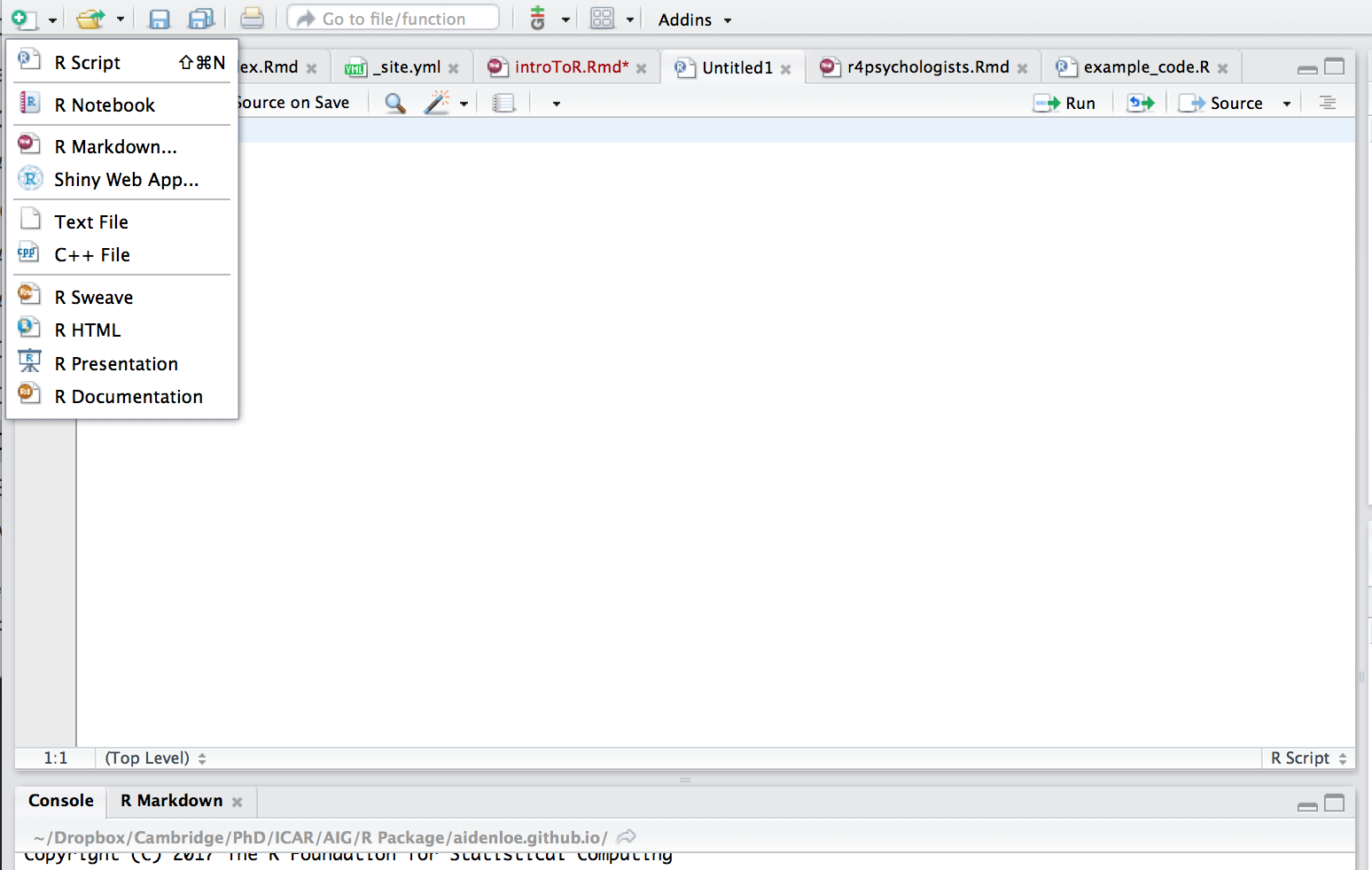
This is an R script file. It is an easy way to record all the steps you take to clean, manipulate and analyse your data. Type all your commands here along with detailed comments - comments are extremely helpful for future reference. You can save, edit and reuse this file as many times as you like. This is also a way of saving your output - you just re-run the code. Thus, its better to create script files than to directly type in the console (bottom left box in RStudio) which is not editable.
Commenting your R script
All code that follows a hash symbol (#) will be ignored by R. i.e. these will be considered comments. It’s best practice to comment your script well so that its easy to come back to even a few months from now, let alone years!
Running R scripts
- Select the lines of code that you want to run and press CTRL+ENTER (Mac users COMMAND+ENTER).
- Run single lines of code (on which your cursor is) by pressing CTRL+ENTER. The cursor will automatically jump to the next line.
- Highlight the lines of code that you want to run and click the ‘Run’ button on the top right corner of the script file in Rstudio.
##------------------------------- Simple Calculations  -------------------------

2+2

x=2+2
x

x-3

3*x

x <- 10 #you can also assign values using this arrow. It's exactly the same as using an = sign. I tend to use =
x
x = x * 2
x
R help! functions and JFGI
(dont know what ‘JFGI’ is?? google it!)
Rstudio’s help commands are a boon. Use it shamelessly!
- help command - help(“FUNCTION_NAME”)
- OR ?FUNCTION_NAME The help command is very useful when you know some functions but know what they do. RStudio will throw up the related documentation.
- ?? command - ??SEARCH The ?? command is more generalised and works well if you dont even know whether a specific function exists. You can just search for terms and RStudio will suggest related functions that you can explore.
The help text will appear in the Rstudio window on the bottom right.
Anything you’re trying to achieve has already been attempted by others throughout the world. Take advantage of it by google-ing your question. There are numerous blogs, forums, tutorials and books with R code that you can just copy/paste and use.
help("insert package name")
mean
??bind
Working Directory
Your “working directory” is the “folder” where R loads and saves data from in this session.
You can change this location so that its convenient to access your files.
The ‘get working directory’ command will show what your working directory is currently set to.
The easiest way to do it in R Studio is to do it through the menus:
Go to Session -> Set working directory -> Choose directory…
getwd() #get current WD
setwd("~/desktop") #set Work Directory
Installing and Loading Packages
You need to install a package only once.
You will have to do it again if you update R
You will need to load the package each time you start an R session. Two approaches to do this.
install.packages("ggplot2")

library(ggplot2)
#     OR
require("ggplot2")
Variables in R
We store data in R by putting the data into a variable
object = "data"
object

numbers = 1:10 # 1 to 10
numbers

object = c(3,4,5,2,2,5,3,7,7,8,9)    # c() is a function that means 'combine'
object
Data Structures
R has different types of data structures:
- Vectors
- Matrices
- Lists
- Data Frames
Vectors
vector1 <- c("A", "B", "C")
vector1[3] #refer to the third element in the vector
vector1[1:2] #refer to elements 1 to 2 in the vector
length(vector1) #function to get the total length of the vector
class(vector1) #what variable type is in the vector?


vector2 <- c(5,1,-7,-1,0)
vector2
class(vector2)


## R performs mathematical calculations on numeric objects
vector3<- c(1:5)
vector3
vector3 = vector3 * 2
vector3

# You can also replace a particular element of a vector using square brackets
vector3[3]
vector3[3] <- 106
vector3
Matrix
# a set of elements that are all the same type, but with rows and columns

sample1 <- matrix(c(1,2,4,4,7,5), nrow=2, byrow = T) #create the matrix
head(sample1) # see first 6 rows
tail(sample1) # see last 6 rows
class(sample1) # see data type

sample1[1,2] #refer to specific elements using square brackets. The first number is the row and the second is the column.
sample1[1,] #if you leave one of them blank, you get the whole row or the whole column. So in this case we have row 1
sample1[,2] #In this case we have column 2


sample2 <- matrix(c(4,7,9,3,7,1,8,2,8,4), ncol=5)
sample2

sample3 <- matrix(c(4,7,9,3,7,1,8,2,8,4), nrow=2)
sample3

# join/bind matrices together
cbind(sample1, sample2) # c = column-wise. So join by column
rbind(sample3, sample2) # r = row-wise. So join by row

# Assign column names
row_matrix <- rbind(sample3, sample2)
colnames(row_matrix) <- c("Maths","English","Physics","Law","Physical Education") #colnames function sets column names
row_matrix
row_matrix[,"Maths"] #so now you can refer by column name
Lists
# a set of elements that are different data structure put together
friend <- list(name="Jasmine", age = 28)
class(friend) # see data type

friend[["age"]] #Double square brackets to refer to a named list element
friend$name #This also works, but it's less safe than the double brackets method
friend[[2]] #or you can refer to the number of the element
length(friend) #how many elements in the list
Data frame
# similar to a matrix, but different class
# a set of elements that are all the same type, but with rows and columns

family <- data.frame(Names=c('John', 'Jane','Paul','Mary'),
           Age=c('28', '72', '86', '32'),
           Gender=c(0,1,0,1))
head(family) # see first 6 rows
tail(family) # see last 6 rows
class(family) # see data type

family$Names #selecting specific columns by names
Load dataset
Loading your data into R studio is perhaps the most important part.
We will use an online example dataset that is in my dropbox folder.
The link below will show you how to automatically download datasets from dropbox using Rstudio. (http://stackoverflow.com/questions/35931923/read-csv-file-from-dropbox-and-plot-it-on-leaflet-map-in-shiny-app)
Note: If your dataset is in your computer, you have to first set the working directory to where you saved “dataset1.csv”. Otherwise you’ll get an error saying: cannot open file ‘dataset1.csv’: No such file or directory. If you don’t know how to do that, go to Working Directory section.
R.Version()$version.string #check R version

df <- read.csv('https://www.dropbox.com/s/lvzw37tkw9y5vnq/dataset1.csv?raw=1')
We will work with csv files for simplicity.
If your dataset (csv file) is in your local folder.
- file argument is the name of your dataset.
- header argument tells R that the first row is the column names
dataset <- read.csv(file = 'Dataset Name.csv', header=TRUE)Dealing with Variables
Here are some useful functions that will give you a feel for datasets you load into R
## Some useful commands that will quickly give you a feel for datasets you load into R
head(df)  # first 6 observations, top of dataset
dim(df)   # the dimensions of the dataset (how many rows by columns)
names(df) # variable names. You could also do colnames(ippq)
summary(df) # summary statistics
str(df) # gives the structure of the dataset
class(df) # data frame: different variables (numbers, characters etc.) stuck together in a table.
# imported data are stored in the format of data frame, it looks almost the same as a matrix, but allows different data types (character/numeric/etc.)


## Four ways of accessing data in the same variable
df$job_satisfaction       # By column name (notice the $-sign)
df[["job_satisfaction"]]  # By column name (notice the double brackets)
df[, "job_satisfaction"]  # By column name (notice the comma)
df[, 40]                  # By column number

## How many male/female respondents do we have?
table(df$gender)    # table(data$variable) gives you the frequency table
summary(df$gender)  # summary(data$variable) gives you descriptive stats for that particular variable, NAs represent missing values. It works with categorical variable...
summary(df$happiness_at_work) # ...as well as continuous variable
Variable calculation
Variable calculation
Lets do some calculations on the variable “job_satisfaction”
- What is the mean/average score of ‘job_satisfaction’?
- What is the mean/average score of ‘job_satisfaction’ for males?
- Is there a significant differences in the average score of ‘job_satisfaction’ between males and females?
#Find the average score of 'job_satisfaction'
mean(df$job_satisfaction)  # Doesn't work if NAs exist in the dataset
mean(df$job_satisfaction, na.rm = T) # Exclude NAs when calculating the average

## Recode variable.
## Lets convert gender into 0 = female, 1 = male
df$is_male <- NA #create a new variable called is_male, and set it to NA for every row
df[df$gender=="male", ]$is_male <- 1  # if gender equals to male, assign 1
df[!df$gender=="male", ]$is_male <- 0 # Notice the '!' just after the opening square bracket. If gender does not equal to male, assign 0
df$is_male

## What's the average job satisfaction  at work for men?
# Option 1
# get a dataset of just men
men = df[df$is_male == 1,]
# calculate mean job satisfaction
mean(df$job_satisfaction, na.rm=T) #average male job satisfaction at work

# Option 2 (functions within functions)
# this does exactly the same thing in a single line of code, and has the advantage of not copying the data into a new variable
mean(df$job_satisfaction[df$is_male == 1], na.rm = T)


# Option 3 (Piping)
# passing the output from one function to the next
require(dplyr) # need this package to use the '%>%'
mean(df$job_satisfaction[df$is_male == 1], na.rm = T)
df$job_satisfaction[df$is_male == 1] %>% mean(na.rm=T)

#Question 4
## Are women statistically more satisfied in their jobs than men at work?
# do a t-test to compare job satisfaction of women vs. men
t.test(x=df$job_satisfaction[df$is_male == 1], y=df$job_satisfaction[df$is_male == 0])
Questions
Here are some questions for you to answer.
First. Go to http://personality-testing.info/_rawdata/
- You can download the Rosenburg Self-Esteem Questionnaire Scale dataset
- Click on ‘RSE’ located in the last column
- A codebook is provided that gives an explanation of the dataset
Make sure to set your working directory to where you saved the dataset!
- Load dataset into R studio.
- How many variables are there in the dataset?
- How many participants are there in the dataset?
- Convert all 0s to NAs. (google!)
- Remove all NAs fom the dataset.
- How many participants are left in the dataset?
- Subset the dataset. (google!)
- Data contains only males information
- Data contains only females information
- Create a new variable in the dataset for total score. [e.g. use rowMeans()]
- What is the average score of self-esteem?
- What is the average score of self-esteem for males?
- What is the average score of self-esteem for females?
- Is there a significant difference between male and female in the self-esteem score?
- Save your R script.
Note: For some, you might need to put the values into separate columns manually in excel. To do this, open the csv file in excel and highlight the entire column 1 (Not just the first cell!).
Go to Data –> Text to Column –> Click “Delimited” –> Check “Tab” –> Click Finish.
This will restructure your data. Making it easier to upload the dataset into R studio.