Web scraping
Aiden Loe
07 January, 2021
Web Scraping (Part 1)
Scraping viewership is one area of web scraping, but perhaps you might be interested in doing sentiment analysis on content.
So we want to extract the contents of the web pages rather than number of times someone viewed the web page.
Scrape content (Wiki)
We will be using the RCurl and XML package to help us with the scraping.
Let’s use the Eurovision_Song_Contest as an example.
The XML package has plenty functions that can allow us to scrape the data.
Usually we are extracting information based on the tags of the web pages.
##### scraping CONTENT OFF WEBSITES ######
require(RCurl)
require(XML)
# XPath is a language for querying XML
# //Select anywhere in the document
# /Select from root
# @select attributes. Used in [] brackets

#### Wikipedia Example ####
url <- "https://en.wikipedia.org/wiki/Eurovision_Song_Contest"
txt = getURL(url) # get the URL html code

# parsing html code into readable format
PARSED <- htmlParse(txt)

# Parsing code using tags
xpathSApply(PARSED, "//h1")

# strops code and return content of the tag
xpathSApply(PARSED, "//h1", xmlValue) # h1 tag
xpathSApply(PARSED, "//h3", xmlValue) # h3 tag
xpathSApply(PARSED, "//a[@href]") # a tag with href attribute


# Go to url
# Highlight references
# right click, inspect element
# Search for tags
xpathSApply(PARSED, "//span[@class='reference-text']",xmlValue) # parse notes and citations
xpathSApply(PARSED, "//cite[@class='citation news']",xmlValue) # parse citation news
xpathSApply(PARSED, "//span[@class='mw-headline']",xmlValue) # parse headlines
xpathSApply(PARSED, "//p",xmlValue) # parsing contents in p tag
xpathSApply(PARSED, "//cite[@class='citation news']/a/@href") # parse links under citation. xmlValue not needed.
xpathSApply(PARSED, "//p/a/@href") # parse href links under all p tags
xpathSApply(PARSED, "//p/a/@*") # parse all atributes under all p tags

# Partial matches - subtle variations within or between pages.
xpathSApply(PARSED, "//cite[starts-with(@class, 'citation news')]",xmlValue) # parse citataion news that starts with..
xpathSApply(PARSED, "//cite[contains(@class, 'citation news')]",xmlValue) # parse citataion news that contains.

# Parsing tree like structure
parsed<-   htmlTreeParse(txt, asText = TRUE)
Scrape content (BBC)
When you know the structure of the data.
All you need to do is to find the correct function to scrape.
##### BBC Example ####
url <- "https://www.bbc.co.uk/news/uk-england-london-46387998"
url <- "https://www.bbc.co.uk/news/education-46382919"
txt = getURL(url) # get the URL html code

# parsing html code into readable format
PARSED <- htmlParse(txt)
xpathSApply(PARSED, "//h1", xmlValue) # h1 tag
xpathSApply(PARSED, "//p", xmlValue) # p tag
xpathSApply(PARSED, "//p[@class='story-body__introduction']", xmlValue) # p tag body
xpathSApply(PARSED, "//div[@class='date date--v2']",xmlValue) # date, only the first is enough
xpathSApply(PARSED, "//meta[@name='OriginalPublicationDate']/@content") # sometimes there is meta data.
Create simple BBC scrapper
Sometimes, creating a function will make your life better and make your script look simpler.
##### Create simple BBC scrapper #####
# scrape title, date and content
BBCscrapper1<- function(url){
  txt = getURL(url) # get the URL html code
  PARSED <- htmlParse(txt) # Parse code into readable format
  title <- xpathSApply(PARSED, "//h1", xmlValue) # h1 tag
  paragraph <- xpathSApply(PARSED, "//p", xmlValue) # p tag
  date <- xpathSApply(PARSED, "//div[@class='date date--v2']",xmlValue) # date, only the first is enough
  if(length(date) == 0){
    date = NA
  }else{
    date <- date[1]
  }

  return(cbind(title,date))
  #return(as.matrix(c(title,date)))
}


# Use function that was just created.
BBCscrapper1("https://www.bbc.co.uk/news/education-46382919")
## title date
## [1,] "Ed Farmer: Expel students who defy initiations ban, says dad" NAKeeping it neat
Using the plyr package helps to arrange the data in an organised way.
## Putting the title and date into a dataframe
require(plyr)
#url
url<- c("https://www.bbc.co.uk/news/uk-england-london-46387998", "https://www.bbc.co.uk/news/education-46382919")
## ldply: For each element of a list, apply function then combine results into a data frame
#put into a dataframe
ldply(url,BBCscrapper1)
## title date
## 1 Man murdered widow, 80, in London allotment row <NA>
## 2 Ed Farmer: Expel students who defy initiations ban, says dad <NA>Web scraping (Part 2)
This example below is taken from code kindly written by David stillwell.
Some editing has been made to the original code.
Scrape from Wiki tables
You have learned how to scrape viewership on wikipedia and content on web pages.
This section is about scraping data tables online.
# Install the packages that you don't have first.
library("RCurl") # Good package for getting things from URLs, including https
library("XML") # Has a good function for parsing HTML data
library("rvest") #another package that is good for web scraping. We use it in the Wikipedia example

#####################
### Get a table of data from Wikipedia
## all of this happens because of the read_html function in the rvest package
# First, grab the page source
us_states = read_html("https://en.wikipedia.org/wiki/List_of_U.S._states_and_territories_by_population") %>% # piping
  # then extract the first node with class of wikitable
  html_node(".wikitable") %>%
  # then convert the HTML table into a data frame
  html_table(fill = TRUE)

# rename
names(us_states)<- c('current rank', '2010 rank', 'state', 'census_population_07_2019', 'census_population_04_2010', 'change_in_percentage', 'change in absolute', "total_US_House_of_Representative_seats", "est_population_per_electoral_vote_2019")

# remove first row
us_states=us_states[-1,]
Scrape from online tables
If we can have two data tables that have at least one column with the same name, then we can merge them together.
The main idea is to link the data together to run simple analysis.
In this case we can get data about funding given to various US states to support building infrastructure to improve students’ ability to walk and bike to school.
######################
url <- "http://apps.saferoutesinfo.org/legislation_funding/state_apportionment.cfm"
funding<-htmlParse(url) #get the data

# find the table on the page and read it into a list object
funding<- readHTMLTable(funding,stringsAsFactors = FALSE)
funding.df <- do.call("rbind", funding) #flatten data

# Contain empty spaces previously.
colnames(funding.df)[1]<- c("state") # shorten colname to just State.

# Match up the tables by State/Territory names
# so we have two data frames, x and y, and we're setting the columns we want to do the matching on by setting by.x and by.y
mydata = merge(us_states, funding.df, by.x="state", by.y="state")
## Warning in merge.data.frame(us_states, funding.df, by.x = "state", by.y =
## "state"): column names 'NA', 'NA', 'NA', 'NA', 'NA', 'NA' are duplicated in the
## resultdim(mydata) # it looks pretty good, but note that we're down to 50 US States, because the others didn't match up by name## [1] 50 25# e.g. "District of Columbia" in the us_states data, doesn't match "Dist. of Col." in the funding data
us_states[!us_states$state %in% funding.df$state,]$state## [1] "Puerto Rico" "District of Columbia"
## [3] "Guam" "U.S. Virgin Islands"
## [5] "Northern Mariana Islands" "American Samoa"
## [7] "Contiguous United States" "The fifty states"
## [9] "The fifty states and D.C." "Total United States"#Replace the total spend column name with a name that's easier to use.
names(mydata)## [1] "state"
## [2] "current rank"
## [3] "2010 rank"
## [4] "census_population_07_2019"
## [5] "census_population_04_2010"
## [6] "change_in_percentage"
## [7] "change in absolute"
## [8] "total_US_House_of_Representative_seats"
## [9] "est_population_per_electoral_vote_2019"
## [10] NA
## [11] NA
## [12] NA
## [13] NA
## [14] NA
## [15] NA
## [16] NA
## [17] "Actual 2005\n\t\t\t \t\t "
## [18] "Actual 2006*\n\t\t\t \t\t "
## [19] "Actual 2007\n\t\t\t \t\t "
## [20] "Actual 2008\n\t\t\t \t\t "
## [21] "Actual 2009\n\t\t\t \t\t "
## [22] "Actual 2010\n\t\t\t \t\t "
## [23] "Actual 2011\n\t\t\t \t\t "
## [24] "Actual 2012\n\t\t\t \t\t "
## [25] "Total\n\t\t \t\t "colnames(mydata)[18] = "total_spend" # year of 2010
names(mydata)## [1] "state"
## [2] "current rank"
## [3] "2010 rank"
## [4] "census_population_07_2019"
## [5] "census_population_04_2010"
## [6] "change_in_percentage"
## [7] "change in absolute"
## [8] "total_US_House_of_Representative_seats"
## [9] "est_population_per_electoral_vote_2019"
## [10] NA
## [11] NA
## [12] NA
## [13] NA
## [14] NA
## [15] NA
## [16] NA
## [17] "Actual 2005\n\t\t\t \t\t "
## [18] "total_spend"
## [19] "Actual 2007\n\t\t\t \t\t "
## [20] "Actual 2008\n\t\t\t \t\t "
## [21] "Actual 2009\n\t\t\t \t\t "
## [22] "Actual 2010\n\t\t\t \t\t "
## [23] "Actual 2011\n\t\t\t \t\t "
## [24] "Actual 2012\n\t\t\t \t\t "
## [25] "Total\n\t\t \t\t "head(mydata)## state current rank 2010 rank census_population_07_2019
## 1 Alabama 24 23 4,921,532
## 2 Alaska 49 48 731,158
## 3 Arizona 14 16 7,421,401
## 4 Arkansas 34 33 3,030,522
## 5 California 1 1 39,368,078
## 6 Colorado 21 22 5,807,719
## census_population_04_2010 change_in_percentage change in absolute
## 1 4,779,736 3.0% +141,796
## 2 710,231 2.9% +20,927
## 3 6,392,017 16.1% +1,029,384
## 4 2,915,918 3.9% +114,604
## 5 37,253,956 5.7% +2,114,122
## 6 5,029,196 15.5% +778,523
## total_US_House_of_Representative_seats est_population_per_electoral_vote_2019
## 1 7 1.61%
## 2 1 0.23%
## 3 9 2.07%
## 4 4 0.92%
## 5 53 12.18%
## 6 7 1.61%
## NA NA NA NA NA NA NA
## 1 546,837 703,076 682,819 1.48% 1.53% –0.05% 1.67%
## 2 243,719 731,158 710,231 0.22% 0.23% –0.01% 0.56%
## 3 674,673 824,600 710,224 2.23% 2.04% 0.19% 2.04%
## 4 505,087 757,631 728,980 0.91% 0.93% –0.02% 1.12%
## 5 715,783 742,794 702,905 11.82% 11.91% –0.09% 10.22%
## 6 645,302 829,674 718,457 1.74% 1.61% 0.14% 1.67%
## Actual 2005\n\t\t\t \t\t total_spend
## 1 $1,000,000 $1,313,659
## 2 $1,000,000 $990,000
## 3 $1,000,000 $1,557,644
## 4 $1,000,000 $990,000
## 5 $1,000,000 $11,039,310
## 6 $1,000,000 $1,254,403
## Actual 2007\n\t\t\t \t\t Actual 2008\n\t\t\t \t\t
## 1 $1,767,375 $2,199,717
## 2 $1,000,000 $1,000,000
## 3 $2,228,590 $2,896,828
## 4 $1,027,338 $1,297,202
## 5 $14,832,295 $18,066,131
## 6 $1,679,463 $2,119,802
## Actual 2009\n\t\t\t \t\t Actual 2010\n\t\t\t \t\t
## 1 $2,738,816 $2,738,816
## 2 $1,000,000 $1,000,000
## 3 $3,612,384 $3,612,384
## 4 $1,622,447 $1,622,447
## 5 $22,580,275 $22,580,275
## 6 $2,659,832 $2,659,832
## Actual 2011\n\t\t\t \t\t Actual 2012\n\t\t\t \t\t
## 1 $2,994,316 $2,556,869
## 2 $1,554,670 $933,567
## 3 $3,733,355 $3,372,404
## 4 $1,911,273 $1,514,664
## 5 $25,976,518 $21,080,209
## 6 $3,022,085 $2,483,132
## Total\n\t\t \t\t
## 1 $17,309,568
## 2 $8,478,237
## 3 $22,013,589
## 4 $10,985,371
## 5 $137,155,013
## 6 $16,878,549# We need to remove commas so that R can treat it as a number.
mydata[,"census_population_04_2010"] = gsub(",", "", mydata[,"census_population_04_2010"]) # removes all commas
(mydata[,"census_population_04_2010"] = as.numeric(mydata[,"census_population_04_2010"])) # converts to number data type## [1] 4779736 710231 6392017 2915918 37253956 5029196 3574097 897934
## [9] 18801310 9687653 1360301 1567582 12830632 6483802 3046355 2853118
## [17] 4339367 4533372 1328361 5773552 6547629 9883640 5303925 2967297
## [25] 5988927 989415 1826341 2700551 1316470 8791894 2059179 19378102
## [33] 9535483 672591 11536504 3751351 3831074 12702379 1052567 4625364
## [41] 814180 6346105 25145561 2763885 625741 8001024 6724540 1852994
## [49] 5686986 563626# Now we have to do the same thing with the funding totals
mydata[,"total_spend"] = gsub(",", "", mydata[,"total_spend"]) #this removes all commas
mydata[,"total_spend"] = gsub("\\$", "", mydata[,"total_spend"]) #this removes all dollar signs. We have a \\ because the dollar sign is a special character.
(mydata[,"total_spend"] = as.numeric(mydata[,"total_spend"])) #this converts it to a number data type## [1] 1313659 990000 1557644 990000 11039310 1254403 998325 990000
## [9] 4494278 2578305 990000 990000 3729568 1798399 990000 990000
## [17] 1127212 1404776 990000 1576594 1752904 3009800 1441060 990000
## [25] 1620703 990000 990000 990000 990000 2399056 990000 5114558
## [33] 2333556 990000 3295093 1010647 990000 3345128 990000 1186047
## [41] 990000 1596222 7009094 990000 990000 2024830 1694515 990000
## [49] 1554314 990000# Now we can do the plotting
options(scipen=9999) #stop it showing scientific notation
plot(x=mydata[,"census_population_04_2010"], y=mydata[,"total_spend"], xlab = 'Population', ylab='Total Spending')-1.png)
cor.test(mydata[,"census_population_04_2010"], mydata[,"total_spend"]) # 0.9810979 - big correlation!##
## Pearson's product-moment correlation
##
## data: mydata[, "census_population_04_2010"] and mydata[, "total_spend"]
## t = 35.126, df = 48, p-value < 0.00000000000000022
## alternative hypothesis: true correlation is not equal to 0
## 95 percent confidence interval:
## 0.9667588 0.9892853
## sample estimates:
## cor
## 0.9810979Plot funding data on map
Perhaps it might be more interesting to see how the data is like on a map.
We can utilise map_data function in the ggplot package to help us with that.
Again, with a bit of data manipulation, we can merge the data table that contains the longitude and latitude information together with the funding data across different states.
require(ggplot2)
all_states <- map_data("state") # states
colnames(mydata)[1] <- "state" # rename to states
mydata$state <- tolower(mydata$state) #set all to lower case
Total <- merge(all_states, mydata, by.x="region", by.y = 'state') # merge data
# we have data for delaware but not lat, long data in the maps
i <- which(!unique(all_states$region) %in% mydata$state)

# Plot data
ggplot() +
  geom_polygon(data=Total, aes(x=long, y=lat, group = group, fill=Total$total_spend),colour="white") +
  scale_fill_continuous(low = "thistle2", high = "darkred", guide="colorbar") +
  theme_bw()  +
  labs(fill = "Funding for School" ,title = "Funding for School between 2005 to 2012", x="", y="") +
  scale_y_continuous(breaks=c()) +
  scale_x_continuous(breaks=c()) +
  theme(panel.border =  element_blank(),
        text = element_text(size=20))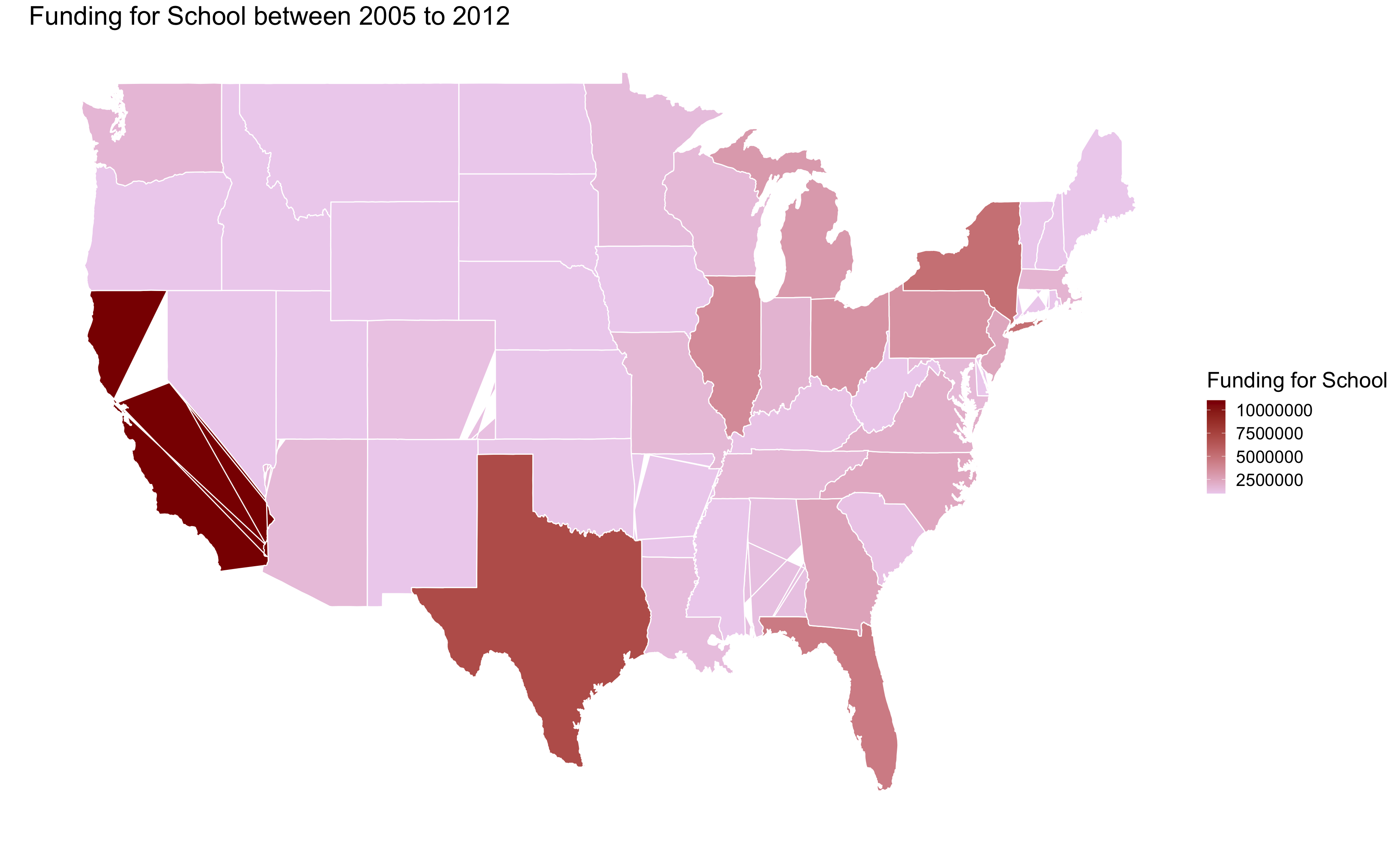
Web scraping (Part 3)
Scrape from discussion forums
Coming soon..